PROBLEM
Customers are very different among themselves. Although each individual has its unique features, it is possible to group them in clusters of similar people that are more likely to respond positively to the same stimulus. This segmentation enables the marketers to give better attention to the selection of customers by adopting different marketing approaches for promotions, prices, communication and products.
Customers are very different among themselves. Although each individual has its unique features, it is possible to group them in clusters of similar people that are more likely to respond positively to the same stimulus. This segmentation enables the marketers to give better attention to the selection of customers by adopting different marketing approaches for promotions, prices, communication and products.
GENERAL Goal
To better understand the different customer segments in order to increase the effectiveness and efficiency of marketing campaigns.
To better understand the different customer segments in order to increase the effectiveness and efficiency of marketing campaigns.
Result
By using statistics, programming and machine learning techniques, it is possible to find patterns hidden in the data. With this information it is possible to build a statistical model that can be used to improve the knowledge about customers’ features and make better strategic decisions regarding product innovation and communication.
By using statistics, programming and machine learning techniques, it is possible to find patterns hidden in the data. With this information it is possible to build a statistical model that can be used to improve the knowledge about customers’ features and make better strategic decisions regarding product innovation and communication.
Short Report
Context
This project was based on a dataset found on Kaggle:
https://www.kaggle.com/arjunbhasin2013/ccdata
It follows the CRISP-DM Methodology.
Tools used:
- Python on Jupyter Notebook
- Power BI
Business Understanding
Credit card companies make the bulk of their money from three things: interest, fees charged to cardholders, and transaction fees paid by businesses that accept credit cards.
With this cluster analysis, we aim at developing a better understanding of the relationships between different groups of consumers that can be used in product positioning, new product and campaign developments and selecting test markets.
Data Understanding
At this stage, we aim at grasping a better knowledge about the different data touch points and dive into the business meaning of the data being leveraged.
The dataset has 18 behavioral variables and summarizes the usage behavior of about 9000 active credit card holders during the last 6 months.
Some of the most relevant variables under analysis were:
- PURCHASES : Total Amount of purchases made by a customer;
- ONEOFFPURCHASES : Maximum purchase amount done in one-go;
- INSTALLMENTSPURCHASES : Amount of purchase done in instalment;
- CASHADVANCE: Amount of cash advance taken out a customer;
- PURCHASESFREQUENCY : How frequently the Purchases are being made;
- ONEOFFPURCHASESFREQUENCY : How frequently Purchases are happening in one-go;
- CASHADVANCEFREQUENCY : How frequently the cash in advance being paid;
We also look at different statistics to get a better sense of the data and detect any anomaly, namely distributions, means, modes, medians, quartiles, maximum and minimum values, identification of missing data, strangely inputted values and variable correlation.
Summary Statistics
Some observations:
- There's a big difference between the average purchase, one-off purchase, installment purchase and cash advance, which indicates skewed distributions;
- Most values for frequency (except purchases are low, which means that most people don't use the card all that much;
- Most people don't fulfill their debt full payment by large;
- Tenure time is pretty much the same for all customers.

Histograms for some of the most relevant features

Histograms for some of the most relevant features

Histograms for some of the most relevant features
The plots visualization confirms the previous assumptions - this kind of distributions also tend to include plenty of extreme values (outliers) which might interfere with our model. In addition, we can also see that there are two distinct group of customers in terms of Purchase frequency.
Another plot tells us that people with a higher credit card limit tend to have high average spending in all credit card features.
Pearson Correlation Heat-map
Correlation coefficient
Correlation ranges from -1 to +1. Values closer to zero mean there is no linear trend between the two variables. The close to 1 the correlation is the more positively correlated they are, if one increases so does the other. The inverse happens for correlations closer to -1, negative correlation, if one decreases the other increases.
We can see that there are plenty of correlated varibales (it was defined a threhold of 0.8 from which variables are considerate highly correlated (namely the pairs: PURCHASES and ONEOFF_PURCHASES, PURCHASES_FREQUENCY and PURCHASES_INSTALLMENTS_FREQUENCY or CASH_ADVANCE_TRX and CASH_ADVANCE_FREQUENCY.
This might be a problem for clustering models because when variables are collinear, some variables get a higher weight than others. If two variables are perfectly correlated, they effectively represent the same concept. But that concept is now represented twice in the data and which gives it twice the weight of all the other variables.
Data Preparation
After the analysis of the dataset, is time to get the data ready for modeling.
At this stage, we perform things such as:
1) missing values (aka data that is missing from our dataset) and define a strategy for dealing with it, which simplistically can be either remove or to impute values;
2) extreme values, the so-called outliers, and the skewness of the distributions, depending on the model we intent to use;
3) feature engineering, which the creation of new variables from the variable we have in hand. In the case, some were created:
- Fee_Applied, that was created to find the clients that would be paying extra fees for not fulfilling their minimum payments.
- Frequency of card usage, which derives from the sum of purchase frequency and cash-advance variables
- Fee_Applied, that was created to find the clients that would be paying extra fees for not fulfilling their minimum payments.
- Frequency of card usage, which derives from the sum of purchase frequency and cash-advance variables
4) Principal Component Analysis – the goal of this process is to reduce the number of variables of a data set, while preserving as much information as possible. It also allows us to have a sneak pick at which seem to be the most defining variables for the clusters’ formation.
Modelling
In this projected, I tested 3 models:
• Hierarchical clustering;
•K-means with PCA;
• K-means;
K-means algorithm is an iterative algorithm that tries to partition the dataset into a per-defined distinct non-overlapping clusters where each data point belongs to only one group.
Example of how K-means workS (source: javatpoint )
Evaluation
From all the models tested, the most reliable on was the third: K-Means without PCA. This was the model which defined the most distinct clusters and understandable clusters based on domain knowledge, intrinsic and extrinsic measures.
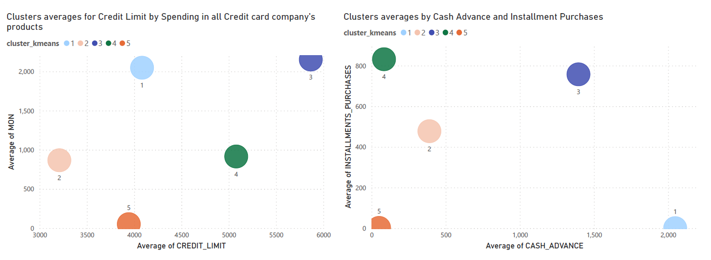
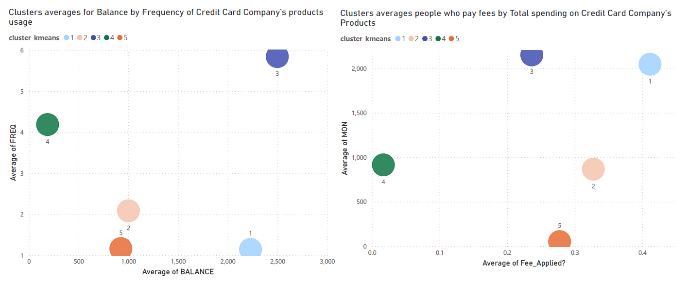
Based on the results of this algorithm, it was possible to identify and clearly define 5 different segments of customers.
Cluster 1: Cash Caged
• People that only use the card for cash-advance and rarely fulfill their debt’s payments, which means they pay a lot of extra fees.
• People that only use the card for cash-advance and rarely fulfill their debt’s payments, which means they pay a lot of extra fees.
Cluster 2: Shopping Club
• People who use their card with a high frequency and mostly for purchases. Most of them pay their minimum payments on time.
• People who use their card with a high frequency and mostly for purchases. Most of them pay their minimum payments on time.
Cluster 3: Debt Scared
• People who don’t use their credit card a lot and, when they do, they pay everything upfront without ever running into dept.
• People who don’t use their credit card a lot and, when they do, they pay everything upfront without ever running into dept.
Cluster 4: Credit Lovers
• People with high credit card limit, who use every feature of the card a lot and rarely pay their dept in full. Nevertheless, they pay their dept on time. Traditionally, the clients who bring more profit with low risk.
• People with high credit card limit, who use every feature of the card a lot and rarely pay their dept in full. Nevertheless, they pay their dept on time. Traditionally, the clients who bring more profit with low risk.
Cluster 5: Loss Leaders
• People who don’t use their card a lot and, when they do, usually they don’t pay their debts on time.
• People who don’t use their card a lot and, when they do, usually they don’t pay their debts on time.
Plotting Differences between each cluster

Plots for Cluster's Average Values in some of the features


